CURVEFIT1D and CURVEFIT1DT

CURVEFIT1D and CURVEFIT1DT

CURVEFIT1D and CURVEFIT1DT are built-in procedures that provide the parameters and statistics resulting from a linear regression curve fit to data. CURVEITFIT1D uses data provided in array variables for the curve fit whereas CURVEFIT1DT uses data from a Lookup table. These procedures provide the same capability as the Curve Fit menu item but it may be more convenient in that the data do not first have to be plotted and the curve fit parameters are returned so that they can be used in following equations.

Format of the CURVEFIT1D Procedure

Call CURVEFIT1D(FitType$, X[1..n], Y[1..n]: a[1..m], RMS, Bias, R|2, a_stderr[1..m])

FitType$ is a string constant or string variable that can be any of the following:

'LINEAR' {fit is Y[i]=a[0]+a[1]*X[i]}

'POLYNOMIAL1' or 'POLY1' {same as linear}

'POLYNOMIAL2' or 'POLY2' {fit is Y[i]=a[0]+a[1]*X[i]+a[2]*X[i]^2}

'POLYNOMIAL3' or 'POLY3' {fit is Y[i]=a[0]+a[1]*X[i]+a[2]*X[i]^2+a[3]*X[i]^3}

'POLYNOMIAL4' or 'POLY4' {fit is Y[i]=a[0]+a[1]*X[i]+a[2]*X[i]^2+a[3]*X[i]^3+a[4]*X[i]^4}

'POLYNOMIAL5' or 'POLY5' {fit is Y[i]=a[0]+a[1]*X[i]+a[2]*X[i]^2+a[3]*X[i]^3+a[4]*X[i]^4+a[5]*X[i]^5}

'POLYNOMIAL6' or 'POLY6' {fit is Y[i]=a[0]+a[1]*X[i]+a[2]*X[i]^2+a[3]*X[i]^3+a[4]*X[i]^4+a[5]*XY[i]^5+a[6]*X[i]^6}

'EXPONENTIAL' or 'EXP' {fit is Y[i]=a[0]*exp(a[1]*X[i])}

'POWER' {fit is Y[i]=a[0]*X[i]^a[1]}

'LOGARITHMIC' or 'LOG' {fit is Y[i]=a[0]+a[1]*ln(X[i])}

X[1..n] is an array of values for the independent variable and Y[1..n] is an array of values for the dependent variables. n can be a numerical constant or a previously defined EES variable. The number of data points in the X and Y arrays must be greater than the number of parameters that are being determined and less than 1,000.

a[1..m] is the array of curve fit parameters returned by the CURVEFIT1D procedures. Note that m is equal to 2 for all cases except for the POLYNOMIAL fit types in which m is equal to one greater than the polynomial order. It is not necessary to use array range notation for the curve fit parameters. For example, a[1..2] can be replaced with a0, a1.

All following outputs are optional.

RMS is root mean square error defined as: sqrt((1/n)*sum[(Y-Y`)^2] where n is the number of data points, and Y` is the estimated value of Y.

BIAS is the bias error defined as: (1/n)*sum[(Y-Y`)].

R|2 is the correlation coefficient between Y and X

a_stderr[1..m] is the standard error of the curve fit parameters defined as the square root of the estimated variance of the parameter

Example 1:

N=10

Duplicate i=1,N

x[i]=lookup('Lookup 1',i,'X')

y[i]=lookup('Lookup 1',i,'Y')

End

call curvefit1d('Linear',x[1..N],y[1..N]:a0,a1,rms,bias,R|2,a0_stderr,a1_stderr)

Example 2:

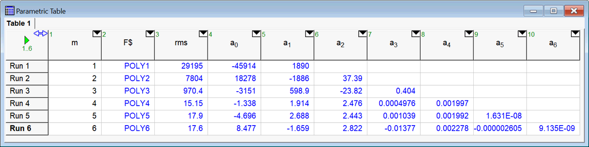
The following example uses a Parametric Table to fit data to polynomials of order 1 through 6. Note the use of the Concat$ and String$ string functions to generate the different polynomial designations.

{m=6} "uncomment this equation when creating the table."

n=100 {n is the number of data points}

F$=concat$('POLY',string$(m)) {m is other order of the polynomial from the table}

Call curvefit1d(F$,X[1..n],Y[1..n]:a[0..m],rms,bias,R|2,a_err[0..m])

Duplicate i=1,n

X[i]=i

Y[i]=i+2.5*X[i]^2+0.002*X[i]^4+random(0,1)*X[i] {fake data for the example}

Y`[i]=a[0]+sum(a[j]*X[i]^j,j=1,m) {predicted value of Y from the polynomial fits}

End

Format of the CURVEFIT1DT Procedure

Call CURVEFIT1DT(FitType$, 'LookupTableName', 'XCOL', 'YCOL', Row1, RowN, doUnits: a[1..m], RMS, Bias, R|2, a_stderr[1..m])

FitType$ is the same as defined above for the CURVEFIT1D procedure.

LookupTableName is a string constant or string variable providing the name of an existing Lookup table or Lookup file (stored on disk).

XCOL is a string constant or string variable providing the name of the column in the Lookup table/file that will provide the values of the independent variables.

YCOL is a string constant or string variable providing the name of the column in the Lookup table/file that will provide the values of the dependent variables.

Row1 is the first row in the table that is used in the curve fit. It can be an integer or previously defined EES variable.

RowN is the last row in the table that is used in the curve fit. It can be an integer or previously defined EES variable.

doUnits is optional. If it is provided, it should be either false# (0) or true# (1). When the dependent and/or independent variables have units, the curve-fit parameters also have associated units. If doUnits is true#, the units of the parameters will be determined and assigned to the a[1..m] parameters. If doUnits is not provided, it is assumed to be false#

The outputs are the same as defined above for the CURVEFIT1D procedure.

Example 3:

A Lookup table with name data contains the following data. The following EES equations provide a power fit

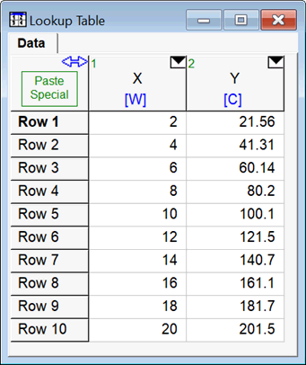
N=10

T$='Data'

X$='X'

Y$='Y'

call curvefit1dt('power',T$,X$,Y$,1,N,false# : a0, a1)

{Solution:

a0=10.72

a1=0.9753}

Example 4:

"This example demonstrates the use of the CurveFit1DT procedure. Saturation pressure versus temperature data are generated and moved to a Lookup Table with the $CopyToLookup directive. The units of the variables are specified with the $VarInfo directive. The CurveFit1DT procedure fits the data to a 2nd order polynomial. The units of the coefficients of the polynomial are determined. Note that the Professional license is needed to run this example."

$UnitSystem SI C kPa

$VarInfo T[] units='C'

$VarInfo P[] units='kPa'

N=10

Duplicate i=1,N

T[i]=10 [C]*i

P[i]=P_sat(Water,T=T[i])

End

$CopyToLookup /T /C /R 'Steam Data' T\C 1, T[1..N]

$CopyToLookup /T /C /R 'Steam Data' P\kPa 1, P[1..N]

$VarInfo P`[] units='kPa'

Call Curvefit1dt('POLY2','Steam Data','T','P',1,N,true# : a0,a1,a2,rms,bias)

Duplicate i=1,N

P`[i]=a0+a1*T[i]+a2*T[i]^2

End

{Solution:

a0=12.75 [kPa]

a1=-0.9215 [kPa/C]

a2=0.01759 [kPa/C^2]

bias=-1.475E-18

N=10

rms=3.161 }