Fast Fourier Transform
The Professional license provides the capability to do transform data in a column in the Lookup table using the Fast Fourier Transform (FFT) algorithm. The following example will illustrate this capability.
First, we will use the EES code below to create a Lookup table with two columns containing time and a measurement at that time. The measurements must be provided at equal increments of time. Note that the data in the Lookup table could have been (and most likely will be) read from a data file having a .txt, .csv, .lkt, or xlsx file name extension. In this case, the data can be read using the $OpenLookup directive or the Open Lookup Table command in the Tables menu.
$UnitSystem Rad
$CheckUnits off
Fs=1000 "sampling frequency"
Tp=1/Fs "sampling period"
L=1500 "length of signal"
DUPLICATE i=1,L
t[i]=i*Tp
S[i]= 0.8 + 0.7*Sin(2*pi*50*t[i]) + sin(2*pi*120*t[i])+Random(-1,1)
END
T$='FFT Test'
N$='time\s'
S$='Signal'
$CopytoLookup /T /R /C T$ N$ 1 t[1..L]
$CopytoLookup /T /R /C T$ S$ 1 S[1..L]
$HideWindow arrays
$ShowWindow Lookup FFT Test
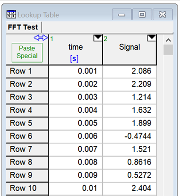
After running this problem, a Lookup table titled FFT test with two columns will appear. The first 10 runs are:
A Fast Fourier Transform of the data in the Signal column is desired. Click on the triangular icon at the upper right of the Signal column and select the FFT Transform radio button.
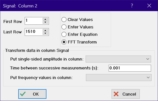
Click in the box adjacent to Put single-sided amplitude in column:
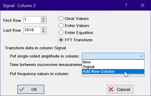
Enter the name of the column that you want the transformed data to appear in or select Add New Column and provide the name for this column.
If you also want to generate a column of frequency values, enter the time between successive measurements in seconds and select (or enter) a name for the column holding the frequency values.
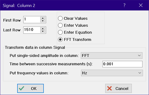
Click OK and the transformed data and frequency data will appear in the designated columns. A plot of the transformed data in column FFT versus the frequency data is shown here.
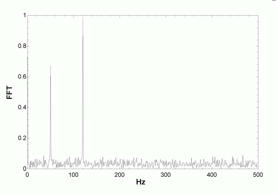
Note that the transformed data (which represent the single-sided amplitude of the complex transform) exhibit three peaks at frequency values of 0, 50 and 120 Hz. These peaks correspond to the steady-state value and the frequencies of the two sine contributions. The amplitudes of these peaks should be 0.8, 0.7 and 1.0, but differ slightly due to the noise in the signal.
Notes:
1. The FFT algorithm requires that the number of data points be a multiple to 2. In this case, 1500 data points were available but only 1024 data points were used in the transform.
2. The FFT algorithm generates real and imaginary numbers. The amplitudes of these values are computed to provide real values.
3. A plot of all of the generated amplitudes would show peaks at high frequencies that are mirror images of the those at the lower frequencies (corresponding to negative frequencies). Only the lower half of the transformed amplitudes are copied in the Lookup table. In this example, that results in the 512 points shown in the plot above.
Back to Change Table Column Values