Curve Fit Table Dialog
The Curve Fit Table Data command allows you to determine a best fit curve through a set of data that are contained in a table. This feature is only available in the Professional version of EES. The curve fit table data implements the curve fitting algorithm described in:
Gavin, H.P.,
"The Levenberg-Marquardt algorithm for nonlinear least squares curve-fitting problems,"
Department of Civil and Environmental Engineering, Duke University,
November 27, 2022. (https://people.duke.edu/~hpgavin/ExperimentalSystems/lm.pdf)
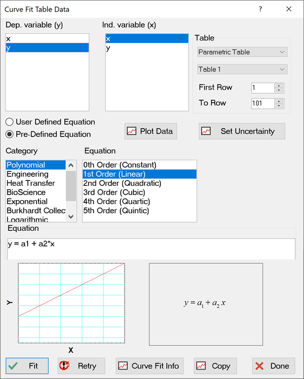
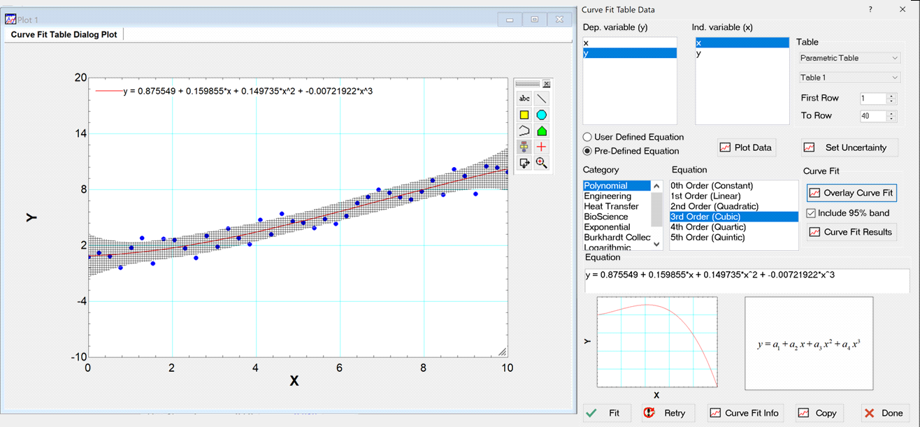
The Curve Fit Table Dialog is shown below.
Choose the source of the data to be fitted by selecting the table and columns at the top of the dialog. Note that the data can reside in either a Parametric or a Lookup Table. Choose the dependent and independent data from the columns in the selected table. The first and last point will be displayed for the column. You can change these values if you wish to curve fit a subset of the data.
The form of the curve fit can either be a pre-defined equation selected from the list or a user-defined function, selected using the radio buttons. The pre-defined equations are broken into categories with some common functions in each category. Selecting a particular curve fit equation causes the associated function, with unknown coefficients (a1, a2, etc.) to be displayed in the Equation Box. An approximate shape of the equation is shown in the left hand box at the bottom and the formatted equation itself to be shown in the right hand box. Alternatively, selecting the User Defined radio button allows the user to enter a functional form in the Equation Box. Note that it is possible to start this process with a pre-defined equation - editing the equation in the Equation Box will cause the selection to shift to User Defined.
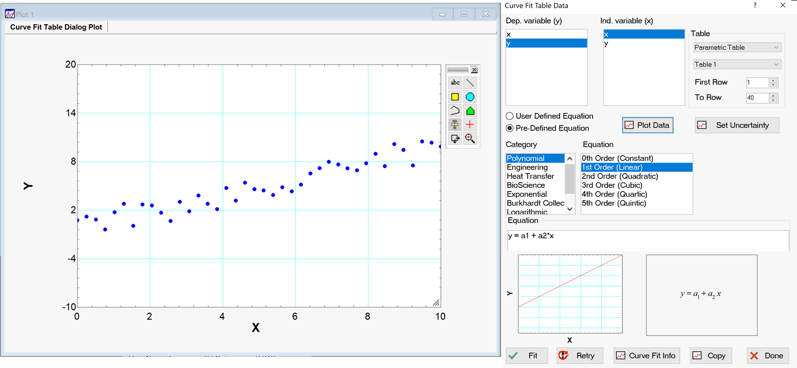
Select the Plot Data button to display the data to be fit on a plot.
Select the Curve Fit Info Button to set the parameters associated with the curve fit in the Curve Fit Table Information dialog. Select the Fit button to initiate the curve fit. If the curve fit was successful then the unknown coefficients in the Equation Box will be changed to their fitted values and the Curve Fit Results button will become enabled. The Retry button will change the equation back to the unknown coefficients. If the data has been plotted then the Overlay Curve Fit button will also be enabled and will cause the best fit curve to be overlaid onto the plotted data. The curve fit equation will also be placed on the plot.
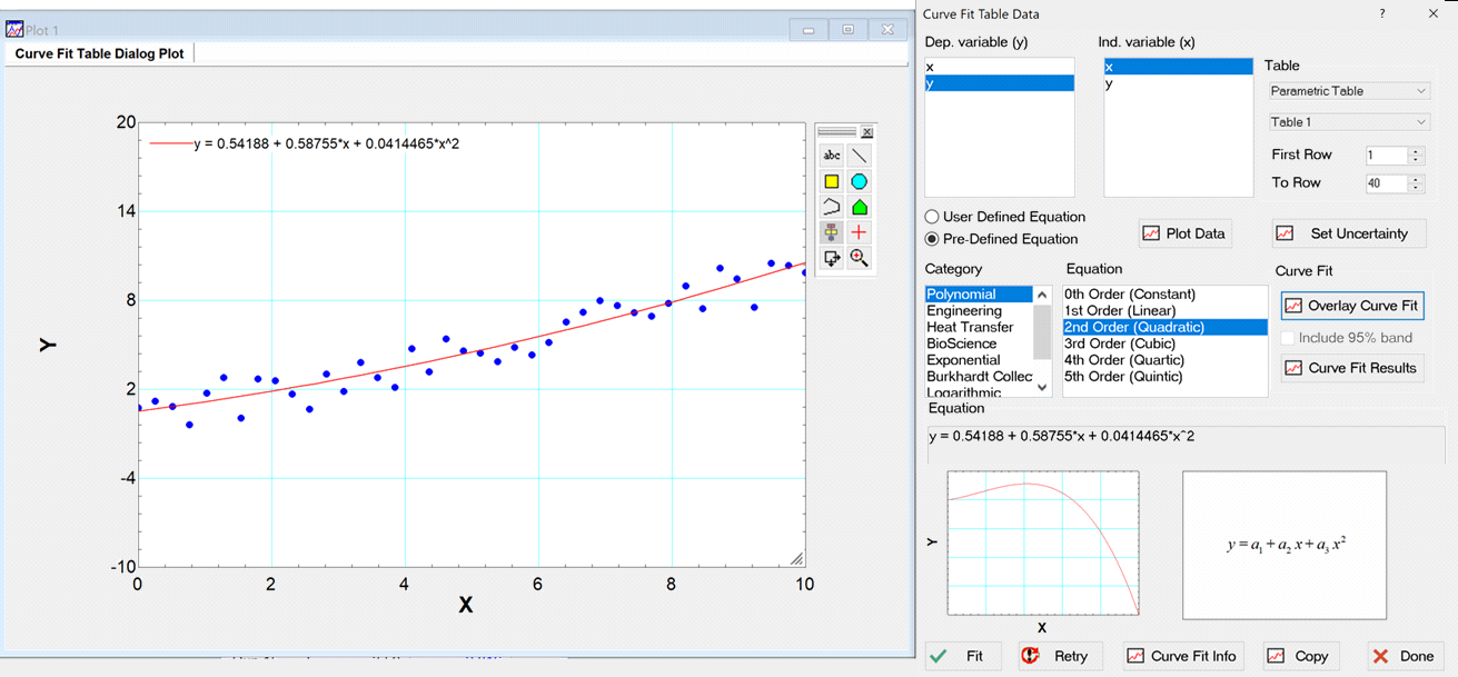
The Copy button will copy the equation to the clipboard allowing it to be pasted as needed. The Curve Fit Results button will bring up the Curve Fit Results dialog that provides statistical information about the curve fit.
It is possible to associate uncertainty with the data in order to weight the use of the data in the curve fitting process by selecting the Set Uncertainty button to bring up the Set Uncertainty dialog. If this is not done then all data are weighted equally.
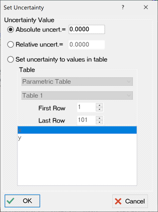
Uncertainty can be set to an absolute value, a relative value, or to values within a table. If values in a Parametric Table have uncertainty associated with them from a previous Uncertainty Table Calculation then these values can be selected as well. Once uncertainty values are provided, they will be used to weight the data during the curve fit process and can also be used to provide a 95% confidence bound for the curve fit by checking the Include 95% band box before selecting Overlay Curve Fit.
See also Curve Fit Plot which is a simpler dialog that can be used to curve fit data from a plot and is available in the Commercial and Professional versions of EES.